3. Sampling the Imaginary

Medium.

We’ll use this helper function to visualize the results of the posterior probability checks:

def plot_ppc(ppc, value=None, vline=None, xvar=None):
    fig, ax = plt.subplots()
    if value:
        ax.axvspan(value - 0.5, value + 0.5, facecolor='grey', alpha=0.35)
    if vline:
        plt.axvline(vline, color='#d55e00', linewidth=3, label='Actual # of Boys')
        plt.legend()
    ax.hist(ppc, bins=100)
    plt.xlabel(f'# of {xvar} Observations')
    plt.ylabel('Frequency')

3M1. Suppose the globe tossing data had turned out to be 8 water in 15 tosses. Construct the posterior distribution, using grid approximation. Use the same flat prior as before.

var = 'Water'
prior = np.ones(1000)
pg, po, s, t = compute_grid_approximation(prior, success=8, tosses=15)
plt.plot(pg, po)
plt.xlabel(f'Probability of {var}')
plt.ylabel('Density')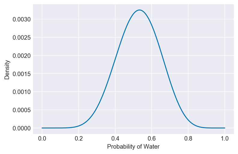

3M1

3M2. Draw 10,000 samples from the grid approximation from above. Then use the samples to calculate the 90% HPDI for p.

np.random.seed(3)
samples = np.random.choice(pg, p=po, size=10000, replace=True)
values = az.hdi(samples, hdi_prob=0.9)
plot_interval(samples, left=values[0], right=values[1], xvar=var)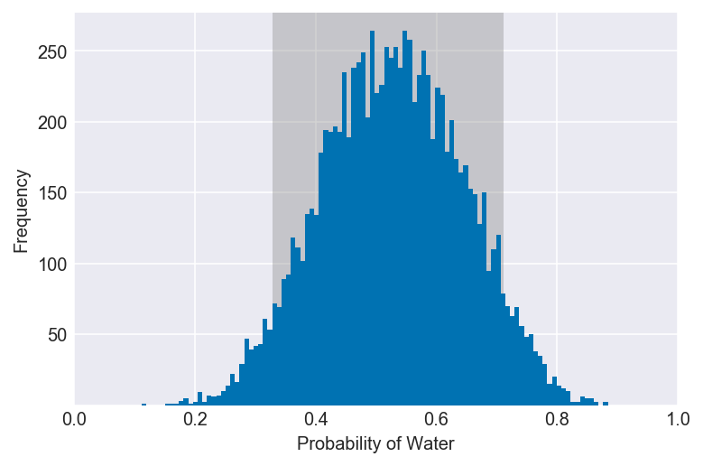

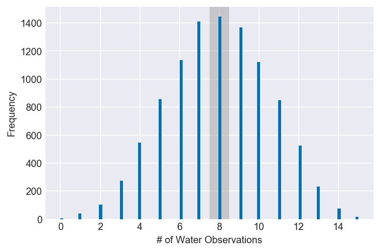
The 90% HDPI for p = [0.329, 0.712]

3M2

3M3. Construct a posterior predictive check for this model and data. This means simulate the distribution of samples, averaging over the posterior uncertainty in p. What is the probability of observing 8 water in 15 tosses?

ppc = stats.binom.rvs(n=15, p=samples, size=10000)
np.mean(ppc == 8)
plot_ppc(ppc, value=8, xvar=var)

Documentation for stats.binom.rvs

p = 0.144

3M3

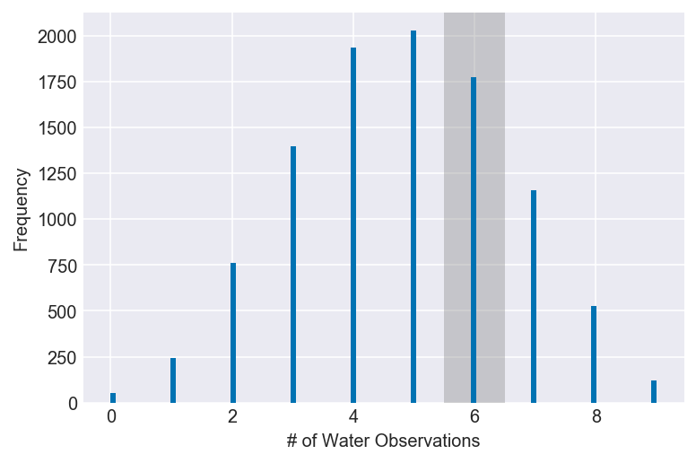
3M4. Using the posterior distribution constructed from the new (8/15) data, now calculate the probability of observing 6 water in 9 tosses.

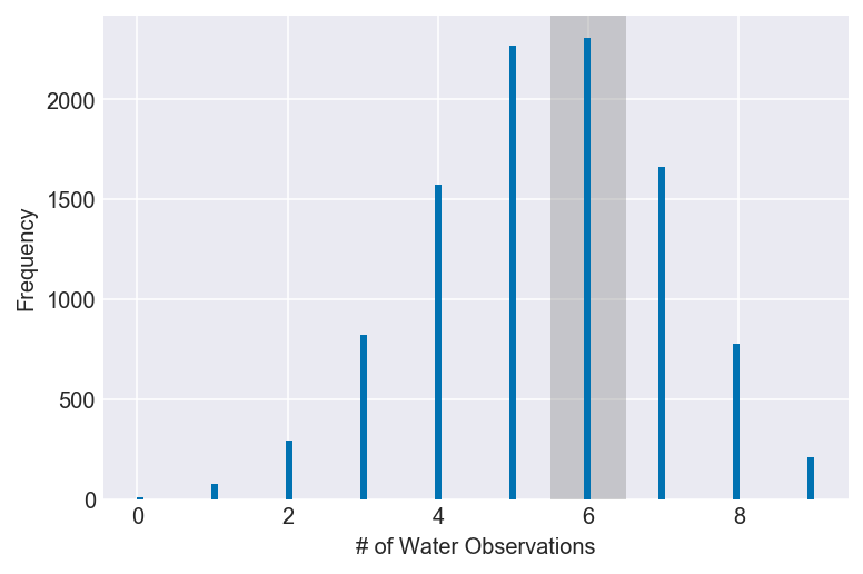
ppc = stats.binom.rvs(n=9, p=samples, size=10000)
np.mean(ppc == 6)
plot_ppc(ppc, value=6, xvar=var)

Documentation for stats.binom.rvs

p = 0.177

3M4

3M5. Start over at 3M1, but now use a prior that is zero below p = 0.5 and a constant above p = 0.5. This corresponds to prior information that a majority of the Earth’s surface is water. Repeat each problem above and compare the inferences. What difference does the better prior make? If it helps, compare inferences (using both priors) to the true value p = 0.7.

prior = np.where(np.linspace(start=0, stop=1, num=1000) < 0.5, 0, 1)
pg, po, s, t = compute_grid_approximation(prior, success=8, tosses=15)
plt.plot(pg, po)
plt.xlabel(f'Probability of {var}')
plt.ylabel('Density')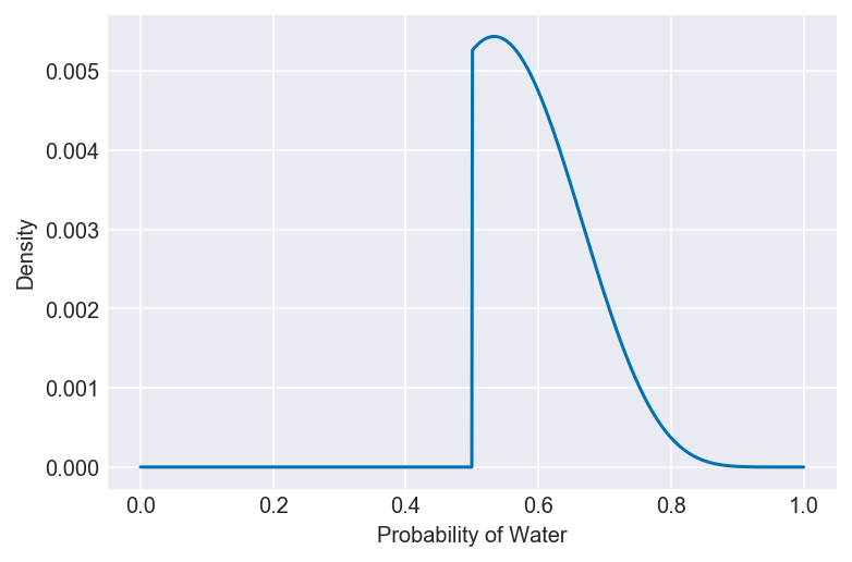

3M5a

np.random.seed(3)
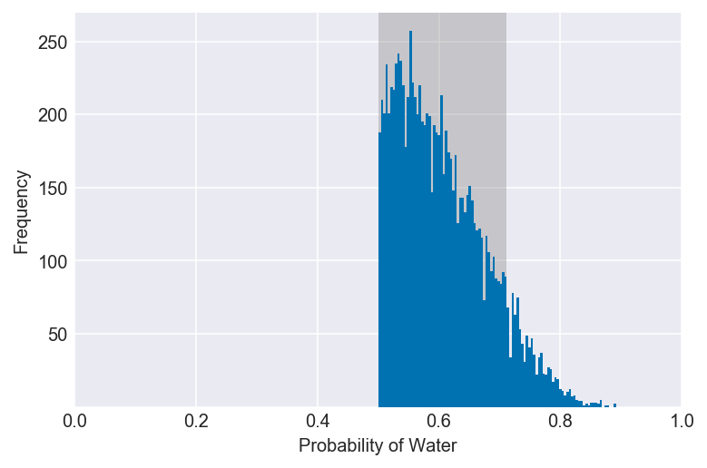
samples = np.random.choice(pg, p=po, size=10000, replace=True)
values = az.hdi(samples, hdi_prob=0.9)
plot_interval(samples, left=values[0], right=values[1], xvar=var)

The 90% HDPI for p = [0.501, 0.711]

Because the new prior assumes that values below 0.5 are impossible, the left interval now begins at that value. Despite this prior, the greatest density of the posterior distribution still falls below a value of approximately 70%, given the data.

3M5b

ppc = stats.binom.rvs(n=15, p=samples, size=10000)
np.mean(ppc == 8)
plot_ppc(ppc, value=8, xvar=var)

p = 0.156

Because the new prior gives higher probabilities to values above 0.5, the probability of observing eight waters in fifteen tosses has grown, though only very slightly. More noticeable is that observing more than or fewer than eight waters has grown more and less probable, respectively.

3M5c

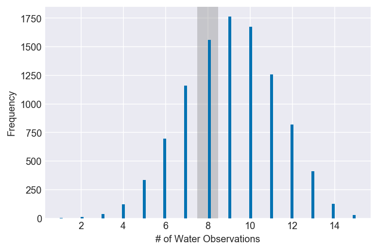
ppc = stats.binom.rvs(n=9, p=samples, size=10000)
np.mean(ppc == 6)
plot_ppc(ppc, value=6, xvar=var)

p = 0.231

The same probabilistic shift towards higher values influences this inference, but, because there is less data than before, the prior plays a larger role in determining the shape of the posterior, and therefore the probability of observing six waters in nine tosses shows a more pronounced increase.

3M5d

← → Top