3. Sampling the Imaginary

Hard.

The practice problems here all use the data below. These data indicate the gender (male=1, female=0) of officially reported first and second born children in 100 two-child families.

birth1 = (1,0,0,0,1,1,0,1,0,1,0,0,1,1,0,1,1,0,0,0,1,0,0,0,1,0,0,0,0,1,1,1,0,1,0,1,1,1,0,1,0,1,1,0,1,0,0,1,1,0,1,0,0,0,0,0,0,0,1,1,0,1,0,0,1,0,0,0,1,0,0,1,1,1,1,0,1,0,1,1,1,1,1,0,0,1,0,1,1,0,1,0,1,1,1,0,1,1,1,1)
birth2 = (0,1,0,1,0,1,1,1,0,0,1,1,1,1,1,0,0,1,1,1,0,0,1,1,1,0,1,1,1,0,1,1,1,0,1,0,0,1,1,1,1,0,0,1,0,1,1,1,1,1,1,1,1,1,1,1,1,1,1,1,1,0,1,1,0,1,1,0,1,1,1,0,0,0,0,0,0,1,0,0,0,1,1,0,0,1,0,0,1,1,0,0,0,1,1,1,0,0,0,0)

So for example, the first family in the data reported a boy (1) and then a girl (0). The second family reported a girl (0) and then a boy (1). The third family reported two girls.

3H1. Using grid approximation, compute the posterior distribution for the probability of a birth being a boy. Assume a uniform prior probability. Which parameter value maximizes the posterior probability?

var = 'Boy'
total = len(birth1 + birth2)
# In order to count the number of boy births,
# we need to count the number of 1's in the data
boys = sum(birth1 + birth2)
prior = np.ones(1000)
pg, po, b, n = compute_grid_approximation(prior, success=boys, tosses=total)
# To find the largest parameter value, we simply need to use the largest value
# in the posterior as an index value
value = pg[po == max(po)]
plt.plot(pg, po)
plt.axvline(value, color='#d55e00', label='Maximum value')
plt.xlabel(f'Probability of {var}')
plt.ylabel('Density')
plt.legend()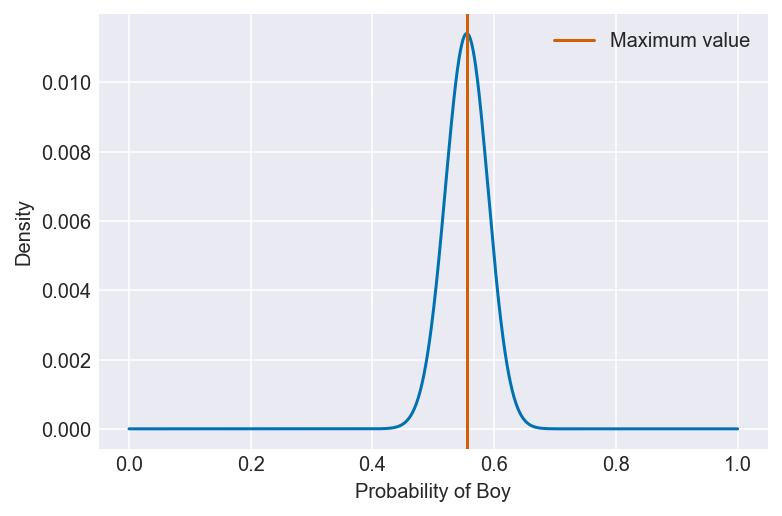

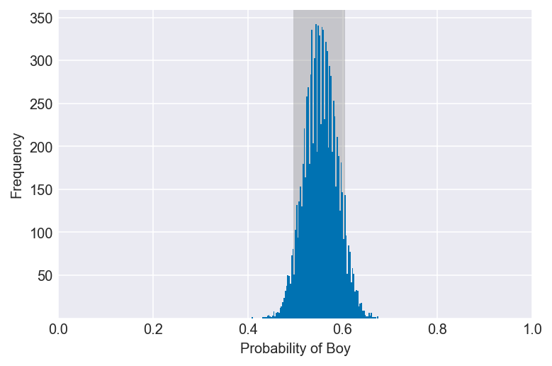
3H2. Using the sample function, draw 10,000 random parameter values from the posterior distribution you calculated above. Use these samples to estimate the 50%, 89%, and 97% highest posterior density intervals.

np.random.seed(3)
samples = np.random.choice(pg, p=po, size=10000, replace=True)
for i in (0.5, 0.89, 0.97):
    values = az.hdi(samples, hdi_prob=i)
    plot_interval(samples, left=values[0], right=values[1], xvar=var)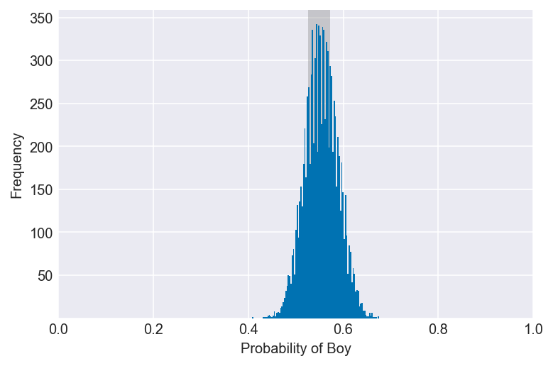

3H3. Use rbinom to simulate 10,000 replicates of 200 births. You should end up with 10,000 numbers, each one a count of boys out of 200 births. Compare the distribution of predicted numbers of boys to the actual count in the data (111 boys out of 200 births). There are many good ways to visualize the simulations, but the dens command (part of the rethinking package) is probably the easiest way in this case. Does it look like the model fits the data well? That is, does the distribution of predictions include the actual observation as a central, likely outcome?

ppc = stats.binom.rvs(n=200, p=samples, size=10000)
plot_ppc(ppc, vline=boys, xvar=var)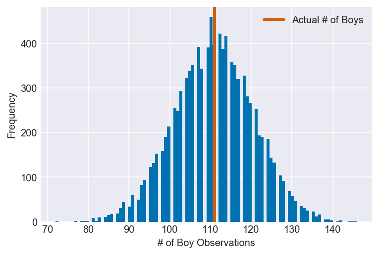

It appears that the model fits the data well, as the number of observed boy births is a central, likely outcome in the model’s simulated data.

3H4. Now compare 10,000 counts of boys from 100 simulated first borns only to the number of boys in the first births, birth1. How does the model look in this light?

I’m assuming that the question is telling us to create a dummy version of the birth1 dataset using the model we created in 3H1, then compare it to the actual data.

boys_1 = sum(birth1)
ppc = stats.binom.rvs(n=100, p=samples, size=10000)
plot_ppc(ppc, vline=boys_1, xvar=var)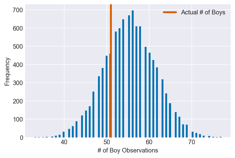

It’s clear that the model overestimates the number of boy births when attempting to recreate the birth1 dataset, though the actual number of observations still lies within a relatively dense area of the predictions. It’s uncertain whether this discrepancy is due to a misspecified model or to the vicissitudes of the birth1 dataset, but providing a more informative prior, gathering more data and looking at the posterior in different ways could help determine which is most likely.

3H5. The model assumes that sex of first and second births are independent. To check this assumption, focus now on second births that followed female first borns. Compare 10,000 simulated counts of boys to only those second births that followed girls. To do this correctly, you need to count the number of first borns who were girls and simulate that many births, 10,000 times. Compare the counts of boys in your simulations to the actual observed count of boys following girls. How does the model look in this light? Any guesses what is going on in these data?

I’m going to assume that the question is telling us to create a dummy version of a subset of the birth2 dataset (boy births that follow girl births) using the model we created in 3H1, then compare it to the actual data.

girls_1 = len(birth1) - sum(birth1)
girl1_boy2 = list(zip(birth1, birth2)).count((0,1))
ppc = stats.binom.rvs(n=girls_1, p=samples, size=10000)
plot_ppc(ppc, vline=girl1_boy2, xvar=var)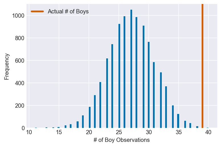

Here we can see that something has gone terribly wrong: the model severely underestimates the number of boy births following girl births. Given that the model assumes that the two datasets are independent, this is reason to believe that they, in fact, are not.

Due to the size of the datasets, we still cannot rule out that this result is due to nothing more than randomness, though that possibility seems to be much less likely now than before. Instead, any number of biological, historical and cultural factors become potential explanations.