3. Sampling the Imaginary

Easy.

The code used to answer the questions below relies on these Python libraries:

import numpy as np
import scipy.stats as stats
import matplotlib.pyplot as plt
import arviz as az

# I'm using this code to make plotting easy in a Jupyter notebook
%matplotlib inline
%config InlineBackend.figure_format = 'retina'
plt.style.use(['seaborn-colorblind', 'seaborn-darkgrid'])

As in Chapter 2, we’ll compute the grid approximation of the posterior distribution using this helper function written by the wonderful people at PyMC3:

def compute_grid_approximation(prior, success=6, tosses=9):
    """
    Parameters:
        prior: np.array
            A distribution representing our state of knowledge
            before seeing the data. The number of items
            should be the same as the number of grid points.
        success: integer
            Number of successes.
            The default is 6.
        tosses: integer
            Number of tosses (i.e. successes + failures).
            The default is 9.
    Returns: 
        p_grid: np.array
            An evenly-spaced parameter grid between 0 and 1.
        posterior: np.array
            The posterior distribution.
    """
    # First, define the parameter grid
    p_grid = np.linspace(0, 1, prior.shape[0])
    # Then compute the likelihood at each point in the grid
    likelihood = stats.binom.pmf(success, tosses, p_grid)
    # Compute the product of the likelihood and the prior
    unstd_posterior = likelihood * prior
    # Finally, standardize the posterior so that it sums to 1
    posterior = unstd_posterior / unstd_posterior.sum()

    return p_grid, posterior, success, tosses

We’ll also use this helper function to visualize the results:

def plot_interval(samples, left=0, right=1, xvar=None):
    fig, ax = plt.subplots()
    ax.axvspan(left, right, facecolor='grey', alpha=0.35)
    ax.hist(samples, bins=100)
    ax.set_xlim(0, 1)
    yt = list((str(int(i)) for i in ax.get_yticks()))
    yt[0] = None
    ax.set_yticklabels(yt)
    plt.xlabel(f'Probability of {xvar}')
    plt.ylabel('Frequency')

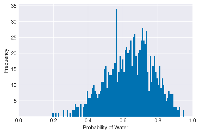
The questions below rely on a set of samples specified in the R code 3.27 box found on p. 69 of Statistical Rethinking. We’ll generate the samples using the following code:

var = 'Water'
size = 1000
# Create a prior distribution of 1000 1's
# This will also create a posterior distribution with 1000 points
prior = np.ones(size)
pg, po, s, t = compute_grid_approximation(prior, success=6, tosses=9)
# Take 1000 samples (with replacement) from the posterior
# The posterior provides the probability for each value in the parameter grid
# Setting a random seed allows the results to be reproducible
np.random.seed(3)
samples = np.random.choice(pg, p=po, size=size, replace=True)
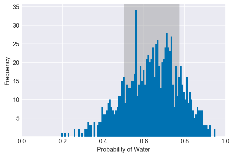
plot_interval(samples, right=0, xvar=var)

Documentation for np.random.seed
Documentation for np.random.choice

3E1. How much posterior probability lies below p = 0.2?

np.mean(samples < 0.2)
plot_interval(samples, right=0.2, xvar=var)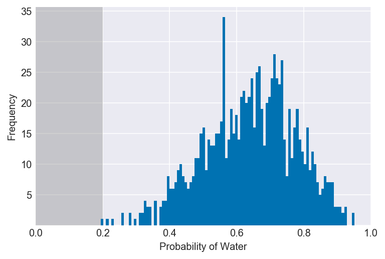

Documentation for np.mean

0.1% lies below 0.2

3E1

3E2. How much posterior probability lies above p = 0.8?

np.mean(samples > 0.8)
plot_interval(samples, left=0.8, xvar=var)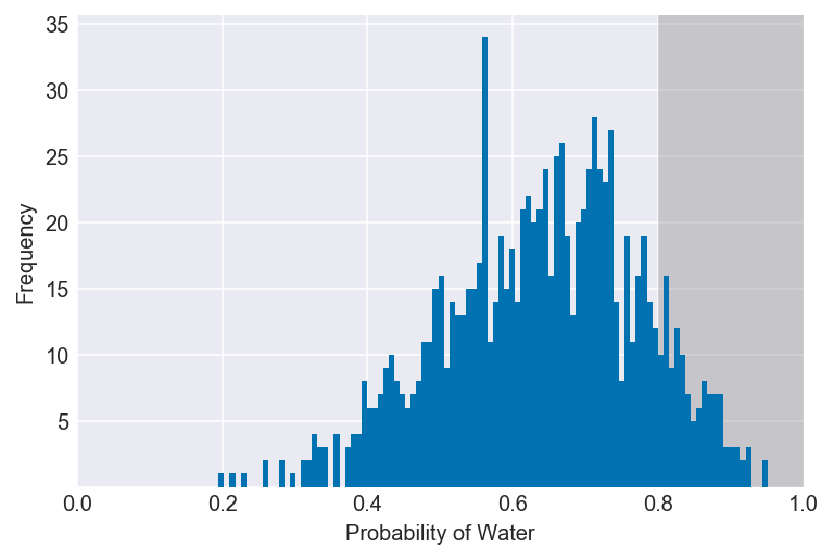

11.9% lies above 0.8

3E2

3E3. How much posterior probability lies between p = 0.2 and p = 0.8?

np.mean((samples > 0.2) & (samples < 0.8))
plot_interval(samples, left=0.2, right=0.8, xvar=var)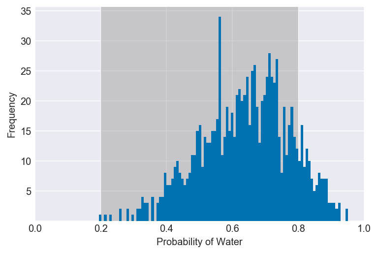

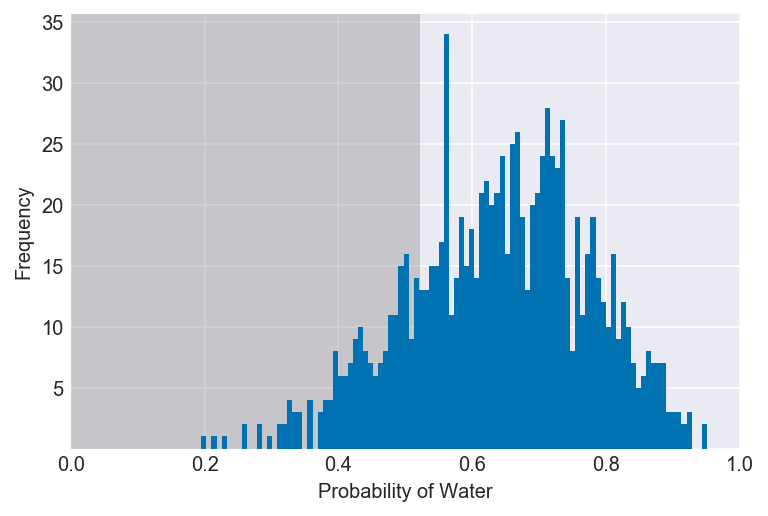
88% lies between 0.2 and 0.8

3E3

3E4. 20% of the posterior probability lies below which value of p?

value = np.percentile(samples, 20)
plot_interval(samples, right=value, xvar=var)

Documentation for np.percentile

p = 0.522

3E4

3E5. 20% of the posterior probability lies above which value of p?

This is equivalent to asking the value of p that lies below 80%.

value = np.percentile(samples, 100-20)
plot_interval(samples, left=value, xvar=var)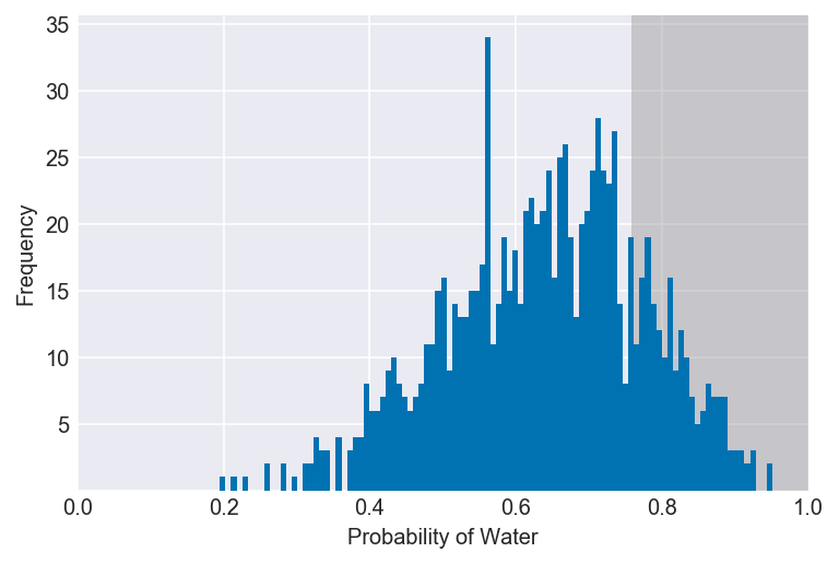

p = 0.758

3E5

3E6. Which values of p contain the narrowest interval equal to 66% of the posterior probability?

values = az.hdi(samples, hdi_prob=0.66)
plot_interval(samples, left=values[0], right=values[1], xvar=var)

Documentation for az.hdi

p = [0.519, 0.782]

3E6

3E7. Which values of p contain 66% of the posterior probability, assuming equal posterior probability both below and above the interval?

If there is an equal posterior probability both below and above the interval, then the remaining intervals comprise the lowest and highest 17% of the posterior (17 + 66 + 17 = 100). We need to compute the interval between those two percentiles.

values = np.percentile(samples, [17, 100-17])
plot_interval(samples, left=values[0], right=values[1], xvar=var)

p = [0.504, 0.774]

3E7

← → Top