2. Small Worlds and Large Worlds
Medium.
The code used to answer some of the questions below relies on these Python libraries:
import numpy as np
import scipy.stats as stats
import matplotlib.pyplot as plt

# I'm using this code to make plotting easy in a Jupyter notebook
%matplotlib inline
%config InlineBackend.figure_format = 'retina'
plt.style.use(['seaborn-colorblind', 'seaborn-darkgrid'])
Moreover, whenever an exercise calls for a grid approximation of the posterior distribution, we’ll compute and plot it using these helper functions written by the wonderful people at PyMC3:
def compute_grid_approximation(prior, success=6, tosses=9):
    """
    Parameters:
        prior: np.array
            A distribution representing our state of knowledge
            before seeing the data. The number of items
            should be the same as the number of grid points.
        success: integer
            Number of successes.
            The default is 6.
        tosses: integer
            Number of tosses (i.e. successes + failures).
            The default is 9.
    Returns:
        p_grid: np.array
            An evenly-spaced parameter grid between 0 and 1.
        posterior: np.array
            The posterior distribution.
    """
    # First, define the parameter grid
    p_grid = np.linspace(0, 1, prior.shape[0])
    # Then compute the likelihood at each point in the grid
    likelihood = stats.binom.pmf(success, tosses, p_grid)
    # Compute the product of the likelihood and the prior
    unstd_posterior = likelihood * prior
    # Finally, standardize the posterior so that it sums to 1
    posterior = unstd_posterior / unstd_posterior.sum()

    return p_grid, posterior, success, tosses

def plot_grid_approximation(p_grid, posterior, success, tosses, x_label):
    """
    This function plots a grid approximation of the posterior distribution.
    """
    plt.plot(p_grid, posterior, 'o-', label=f'Success = {success}\nTosses = {tosses}')
    plt.xlabel(x_label)
    plt.ylabel('Posterior Probability')
    plt.legend(loc=0)
Documentation for np.linspace
Documentation for stats.binom.pmf
You’ll notice that the grid_approximation function is very similar to that in the R code 2.3 box found on p. 40 of Statistical Rethinking.
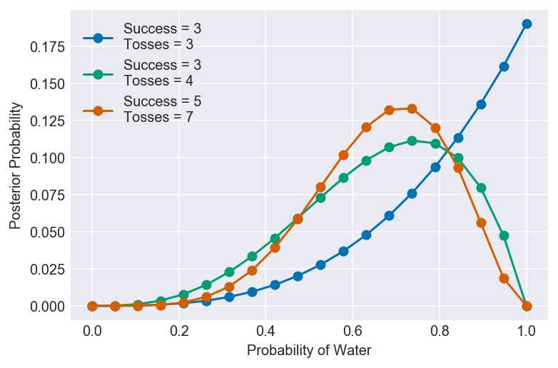
2M1. Recall the globe tossing model from the chapter. Compute and plot the grid approximate posterior distribution for each of the following sets of observations. In each case, assume a uniform prior for p.
- 1) W, W, W
- 2) W, W, W, L
- 3) L, W, W, L, W, W, W
# Create a prior distribution of 20 1's as in Fig 2.7 on pg. 41
# This will also create a posterior distribution with 20 points
prior = np.ones(20)
x_label = 'Probability of Water'
# 1) W, W, W
pg, po, s, t = compute_grid_approximation(prior, success=3, tosses=3)
plot_grid_approximation(pg, po, s, t, x_label)
# 2) W, W, W, L
pg, po, s, t = compute_grid_approximation(prior, success=3, tosses=4)
plot_grid_approximation(pg, po, s, t, x_label)
# 3) L, W, W, L, W, W, W
pg, po, s, t = compute_grid_approximation(prior, success=5, tosses=7)
plot_grid_approximation(pg, po, s, t, x_label)
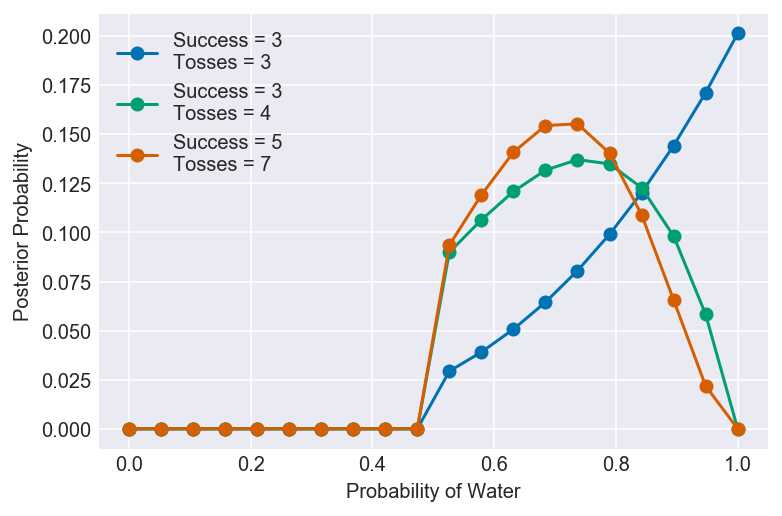
2M2. Now assume a prior for p that is equal to zero when p < 0.5 and is a positive constant when p ≥ 0.5. Again compute and plot the grid approximate posterior distribution for each of the sets of observations in the problem just above.
# Create a distribution of 20 evenly spaced points between 0 and 1
p_grid = np.linspace(start=0, stop=1, num=20)
# Turn every point below 0.5 into a 0; every point above into a 1
prior = np.where(p_grid < 0.5, 0, 1)
x_label = 'Probability of Water'
# 1) W, W, W
pg, po, s, t = compute_grid_approximation(prior, 3, 3)
plot_grid_approximation(pg, po, s, t, x_label)
# 2) W, W, W, L
pg, po, s, t = compute_grid_approximation(prior, 3, 4)
plot_grid_approximation(pg, po, s, t, x_label)
# 3) L, W, W, L, W, W, W
pg, po, s, t = compute_grid_approximation(prior, 5, 7)
plot_grid_approximation(pg, po, s, t, x_label)
2M3. Suppose there are two globes, one for Earth and one for Mars. The Earth globe is 70% covered in water. The Mars globe is 100% land. Further suppose that one of these globes—you don’t know which—was tossed in the air and produced a “land” observation. Assume that each globe was equally likely to be tossed. Show that the posterior probability that the globe was the Earth, conditional on seeing “land” (Pr(Earth | land)), is 0.23.
2M4. Suppose you have a deck with only three cards. Each card has two sides, and each side is either black or white. One card has two black sides. The second card has one black and one white side. The third card has two white sides. Now suppose all three cards are placed in a bag and shuffled. Someone reaches into the bag and pulls out a card and places it flat on a table. A black side is shown facing up, but you don’t know the color of the side facing down. Show that the probability that the other side is also black is $\frac23$. Use the counting method (Section 2 of the chapter) to approach this problem. This means counting up the ways that each card could produce the observed data (a black side facing up on the table).
Given the cards B1/B2, B/W & W/W, three combinations match the observed state:
- 1) B1/B2
- 2) B2/B1
- 3) B/W
Of these three combinations, in only two (1 & 2) is the other side black. Therefore the probability that the side facing down is black, given that the side facing up is black, is $\frac23$.
2M5. Now suppose there are four cards: B/B, B/W, W/W, and another B/B. Again suppose a card is drawn from the bag and a black side appears face up. Again calculate the probability that the other side is black.
Given the cards B1/B2, B/W, W/W & B3/B4, five combinations match the observed state:
- 1) B1/B2
- 2) B2/B1
- 3) B/W
- 4) B3/B4
- 5) B4/B3
Of these five combinations, in only four (1, 2, 4 & 5) is the other side black. Therefore the probability that the side facing down is black, given that the side facing up is black, is $\frac45$.
2M6. Imagine that black ink is heavy, and so cards with black sides are heavier than cards with white sides. As a result, it’s less likely that a card with black sides is pulled from the bag. So again assume there are three cards: BB, B/W, and W/W. After experimenting a number of times, you conclude that for every way to pull the B/B card from the bag, there are 2 ways to pull the B/W car and 3 ways to pull the W/W card. Again suppose that a card is pulled and a black side appears face up. Show that the probability the other side is black is now 0.5. Use the counting method, as before.
When using the counting method, the influence of the black ink effectively adds cards to the deck, in proportion to the likelihood of their being drawn. Unlike in 2M4, our deck now contains the following cards: B1/B2, B/W, B/W, W/W, W/W & W/W. Given these cards, four combinations match the observed state:
- 1) B1/B2
- 2) B2/B1
- 3) B/W
- 4) B/W
Of these four combinations, in only two (1 & 2) is the other side black. Therefore the probability that the side facing down is black, given that the side facing up is black, is $\frac24 = \frac12$.
2M7. Assume again the original card problem, with a single card showing a black side face up. Before looking at the other side, we draw another card from the bag and lay it face up on the table. The face that is shown on the new card is white. Show that the probability that the first card, the one showing a black side, has black on its other side is now 0.75. Use the counting method, if you can. Hint: Treat this like the sequence of globe tosses, counting all the ways to see each observation, for each possible first card.
Given the cards B1/B2, B/W & W1/W2, eight combinations match the observed state:
- 1) B1/B2, W/B
- 2) B1/B2, W1/W2
- 3) B1/B2, W2/W1
- 4) B2/B1, W/B
- 5) B2/B1, W1/W2
- 6) B2/B1, W2/W1
- 7) B/W, W1/W2
- 8) B/W, W2/W1
Of these eight combinations, in only six (1, 2, 3, 4, 5, 6) is the other side of the first card black. Therefore the probability that the facedown side of the first card is black, given that the faceup side of the first card is black, is $\frac68 = \frac34$.